Manuscript LTER Time Series Analysis
Introduction
In the Santa Barbara Channel sub-region of the California Current, aragonite saturation is currently monitored a relatively fine spatial and temporal scale, through the Santa Barbara Coastal Long Term Ecological Research Project (SBC LTER), run by the National Science Foundation, and housed at the University of California, Santa Barbara. The SBC LTER runs four sites that collect aragonite saturation state every twenty minutes, spread across a distance of 50 miles from the Santa Barbara Pier westward to the Gaviota Coast. These sensors are located at the Santa Barbara Pier, Mohawk Reef, Alegria Reef, and Arroyo Quemado Reef (figure 1). As part of the ongoing effort to establish a cohesive OA monitoring network, this project aims to characterize autocorrelation and covariance in the SBC LTER aragonite measurements. This analysis help gain understanding of the spatial and temporal scale of autocorrelation and establish reference points for how frequently aragonite should be measured in coastal environments and how great the distance between measurements can be without losing valuable information between data collection locations. Results help inform future management decisions in how to design an ideal OA monitoring network and how to improve the network that exists today.
Step 1. Setup
Load packages and data
library(lubridate)
library(dplyr)
library(devtools)
library(here)
library(rowr)
library(tidyverse)
library(knitr)

ale <- read_csv("data/ALE_arag.csv")
arq <- read_csv("data/ARQ_arag.csv")
mko <- read_csv("data/MKO_arag.csv")
sbh <- read_csv("data/SBH_arag.csv")
Organize and clean data
Data were obtained through the SBC LTER website (http://sbc.lternet.edu/) and imported into R Studio (version 1.1.419). Here we load LTER data and organize/clean.
lter <- merge.data.frame(ale, arq, by = 'Time_stamp_UTC', all.x = T)
lter <- merge.data.frame(lter, mko, by = 'Time_stamp_UTC', all.x = T)
lter <- merge.data.frame(lter, sbh, by = 'Time_stamp_UTC', all.x = T)

lter[lter == -9999] <- NA

lter <- lter[c(1, 5, 9, 13, 17)]

names(lter) <- c("Time_Stamp_UTC", "Ale_Arag", "Arq_Arag", "Mko_Arag", "Sbh_Arag")
Remove Seasonal Trends
Here we remove the seasonal signal of aragonite saturation (i.e. seasonal upwelling trend) by aggregating data by month and calculating means of these monthly aggregates. Observations were subtracted from these monthly values, and resulting data represents the deviation from the monthly mean.
lter$month <- month(lter$Time_Stamp_UTC)

ale_arag_monthly <- aggregate(Ale_Arag ~ month, lter, mean)
arq_arag_monthly <- aggregate(Arq_Arag ~ month, lter, mean)
mko_arag_monthly <- aggregate(Mko_Arag ~ month, lter, mean)
sbh_arag_monthly <- aggregate(Sbh_Arag ~ month, lter, mean)

ltermerge <- merge.data.frame(lter, ale_arag_monthly, by = 'month', all.x = T)
ltermerge <- merge.data.frame(ltermerge, arq_arag_monthly, by = 'month', all.x = T)
ltermerge <- merge.data.frame(ltermerge, mko_arag_monthly, by = 'month', all.x = T)
ltermerge <- merge.data.frame(ltermerge, sbh_arag_monthly, by = 'month', all.x = T)

ltermerge$ale_res_arag <- ltermerge$Ale_Arag.x-ltermerge$Ale_Arag.y
ltermerge$arq_res_arag <- ltermerge$Arq_Arag.x-ltermerge$Arq_Arag.y
ltermerge$mko_res_arag <- ltermerge$Mko_Arag.x-ltermerge$Mko_Arag.y
ltermerge$sbh_res_arag <- ltermerge$Sbh_Arag.x-ltermerge$Sbh_Arag.y

ltermerge <- ltermerge[order(ltermerge$Time_Stamp_UTC),]

ltermerge <- ltermerge[c(2, 11, 12, 13, 14)]

ltermerge$Time_Stamp_UTC <- as.POSIXct(ltermerge$Time_Stamp_UTC,format = "%Y-%m-%dT %H:%M:%SZ")
Separate Time Chunks
If the four inshore ocean SBC LTER sensors are functioning normally, they measure aragonite saturation state every 20 minutes. However, sensors occasionally require maintenance or replacement, meaning that large chunks of time exist where at least one of the four is not collecting data. In fact, since the sensors were deployed in 2012, there were only several months during which all four sensors were collecting data.
Here, the time series data are split into separate chunks when the time gap between two measurements exceeded 20 minutes (signifying equipment malfunction). We separate the time series for each site into time chunks of continous measurement at 20 minute intervals so that the interval is consistent when calculating autocorrelation
#ale

alearag <- ltermerge[c(1, 2)]

alearag <- na.omit(alearag)

n = length(alearag$Time_stamp_UTC)

alearag$difftime = 0

for (i in 1:nrow(alearag)){
  d <- difftime(alearag$Time_Stamp_UTC[i+1], alearag$Time_Stamp_UTC[i], units = "mins")
  alearag$difftime[i] <- d
}

breaks <- which(alearag$difftime != 20)

ale1 <- alearag[c(1:breaks[1]),]
ale2 <- alearag[c((breaks[1]+1):breaks[2]),]
ale3 <- alearag[c((breaks[2]+1):breaks[3]),]
ale4 <- alearag[c((breaks[3]+1):breaks[4]),]
ale5 <- alearag[c((breaks[4]+1):breaks[5]),]
ale6 <- alearag[c((breaks[5]+1):breaks[6]),]
ale7 <- alearag[c((breaks[6]+1):n),]

#arq

arqarag <- ltermerge[, c(1,3)]

arqarag <- na.omit(arqarag)

n = length(arqarag$Time_Stamp_UTC)

arqarag$difftime = 0

for (i in 1:nrow(arqarag)){
  d <- difftime(arqarag$Time_Stamp_UTC[i+1], arqarag$Time_Stamp_UTC[i])
  arqarag$difftime[i] <- d
}

breaks <- which(arqarag$difftime != 20)

arq1 <- arqarag[c(1:breaks[1]),]
arq2 <- arqarag[c((breaks[1]+1):breaks[2]),]
arq3 <- arqarag[c((breaks[2]+1):n),]

#mko

mkoarag <- ltermerge[, c(1,4)]

mkoarag <- na.omit(mkoarag)

n = length(mkoarag$Time_Stamp_UTC)

mkoarag$difftime = 0

for (i in 1:nrow(mkoarag)){
  d <- difftime(mkoarag$Time_Stamp_UTC[i+1], mkoarag$Time_Stamp_UTC[i])
  mkoarag$difftime[i] <- d
}

breaks <- which(mkoarag$difftime != 20)

mko1 <- mkoarag[c(1:breaks[1]),]
mko2 <- mkoarag[c((breaks[1]+1):breaks[2]),]
mko3 <- mkoarag[c((breaks[2]+1):breaks[3]),]
mko4 <- mkoarag[c((breaks[3]+1):n),]

#sbh

sbharag <- ltermerge[, c(1,5)]

sbharag <- na.omit(sbharag)

n = length(sbharag$Time_Stamp_UTC)

sbharag$difftime = 0

for (i in 1:nrow(sbharag)){
  d <- difftime(sbharag$Time_Stamp_UTC[i+1], sbharag$Time_Stamp_UTC[i])
  sbharag$difftime[i] <- d
}

breaks <- which(sbharag$difftime != 20)

sbh1 <- sbharag[c(1:breaks[1]),]
sbh2 <- sbharag[c((breaks[1]+1):breaks[2]),]
sbh3 <- sbharag[c((breaks[2]+1):breaks[3]),]
sbh4 <- sbharag[c((breaks[3]+1):breaks[4]),]
sbh5 <- sbharag[c((breaks[4]+1):breaks[5]),]
sbh6 <- sbharag[c((breaks[5]+1):n),]
Step 2. Autocorrelation
Calculate Autocorrelation
The autocorrelation is calculated for each of these subsets of the whole time series, with a maximum lag determined by 1/3 the length of the subset, meaning some of these subsets had much longer maximum lags than others. For each lag at each LTER site, the average autocorrelation was calculated with the mean of all time series subsets that were long enough to provide data at that lag – i.e. all subsets could provide information for lag 1 and lag 2, but only subsets that were at least 30 days long could provide information for lags in day 10. Thus, smaller lags are made of averages across all time series subsets, while larger lags rely on data from one or two of the time series subsets. Decorrelation time scales were determined by finding the first zero crossing of the autocorrelation value.
#ale

acf_ale1 <- acf(ale1$ale_res_arag, lag.max = nrow(ale1)/3, type = "correlation", xaxt = "n", xlab='Lag (days)', main = 'Autocorrelation', ylab = '')
axis(1, at=72*(0:50), labels = 1*(0:50))
acf_ale2 <- acf(ale2$ale_res_arag, lag.max = nrow(ale2)/3, type = "correlation", xaxt = "n", xlab='Lag (days)', main = 'Autocorrelation', ylab = '')
axis(1, at=72*(0:50), labels = 1*(0:50)) acf_ale3 <- acf(ale3$ale_res_arag, lag.max = nrow(ale3)/3, type = "correlation", xaxt = "n", xlab='Lag (days)', main = 'Autocorrelation', ylab = '')
axis(1, at=72*(0:50), labels = 1*(0:50)) acf_ale4 <- acf(ale4$ale_res_arag, lag.max = nrow(ale4)/3, type = "correlation", xaxt = "n", xlab='Lag (days)', main = 'Autocorrelation', ylab = '')
axis(1, at=72*(0:50), labels = 1*(0:50)) acf_ale5 <- acf(ale5$ale_res_arag, lag.max = nrow(ale5)/3, type = "correlation", xaxt = "n", xlab='Lag (days)', main = 'Autocorrelation', ylab = '')
axis(1, at=72*(0:50), labels = 1*(0:50)) acf_ale6 <- acf(ale6$ale_res_arag, lag.max = nrow(ale6)/3, type = "correlation", xaxt = "n", xlab='Lag (days)', main = 'Autocorrelation', ylab = '')
axis(1, at=72*(0:50), labels = 1*(0:50)) acf_ale7 <- acf(ale7$ale_res_arag, lag.max = nrow(ale7)/3, type = "correlation", xaxt = "n", xlab='Lag (days)', main = 'Autocorrelation', ylab = '')
axis(1, at=72*(0:50), labels = 1*(0:50)) acf_ale1_df <- acf_ale1[["acf"]]
acf_ale2_df <- acf_ale2[["acf"]]
acf_ale3_df <- acf_ale3[["acf"]]
acf_ale4_df <- acf_ale4[["acf"]]
acf_ale5_df <- acf_ale5[["acf"]]
acf_ale6_df <- acf_ale6[["acf"]]
acf_ale7_df <- acf_ale7[["acf"]]
acf_ale_tot <- cbind.fill(acf_ale1_df, acf_ale2_df, acf_ale3_df, acf_ale4_df, acf_ale5_df, acf_ale6_df, acf_ale7_df, fill = NA)
acf_ale_final <- rowMeans(acf_ale_tot, na.rm = TRUE)
#arq
acf_arq1 <- acf(arq1$arq_res_arag, lag.max = nrow(ale1)/3, type = "correlation", xaxt = "n", xlab='Lag (days)', main = 'Autocorrelation', ylab = '')
axis(1, at=72*(0:50), labels = 1*(0:50)) acf_arq2 <- acf(arq2$arq_res_arag, lag.max = nrow(ale2)/3, type = "correlation", xaxt = "n", xlab='Lag (days)', main = 'Autocorrelation', ylab = '')
axis(1, at=72*(0:50), labels = 1*(0:50)) acf_arq3 <- acf(arq3$arq_res_arag, lag.max = nrow(ale3)/3, type = "correlation", xaxt = "n", xlab='Lag (days)', main = 'Autocorrelation', ylab = '')
axis(1, at=72*(0:50), labels = 1*(0:50)) acf_arq1_df <- acf_arq1[["acf"]]
acf_arq2_df <- acf_arq2[["acf"]]
acf_arq3_df <- acf_arq3[["acf"]]
acf_arq_tot <- cbind.fill(acf_arq1_df, acf_arq2_df, acf_arq3_df, fill = NA)
acf_arq_final <- rowMeans(acf_arq_tot, na.rm = TRUE)
#mko
acf_mko1 <- acf(mko1$mko_res_arag, lag.max = nrow(mko1)/3, type = "correlation", xaxt = "n", xlab='Lag (days)', main = 'Autocorrelation', ylab = '')
axis(1, at=72*(0:30), labels = 1*(0:30)) acf_mko2 <- acf(mko2$mko_res_arag, lag.max = nrow(mko2)/3, type = "correlation", xaxt = "n", xlab='Lag (days)', main = 'Autocorrelation', ylab = '')
axis(1, at=72*(0:30), labels = 1*(0:30)) acf_mko3 <- acf(mko3$mko_res_arag, lag.max = nrow(mko3)/3, type = "correlation", xaxt = "n", xlab='Lag (days)', main = 'Autocorrelation', ylab = '')
axis(1, at=72*(0:30), labels = 1*(0:30)) acf_mko4 <- acf(mko4$mko_res_arag, lag.max = nrow(mko4)/3, type = "correlation", xaxt = "n", xlab='Lag (days)', main = 'Autocorrelation', ylab = '')
axis(1, at=72*(0:30), labels = 1*(0:30)) acf_mko1_df <- acf_mko1[["acf"]]
acf_mko2_df <- acf_mko2[["acf"]]
acf_mko3_df <- acf_mko3[["acf"]]
acf_mko4_df <- acf_mko4[["acf"]]
acf_mko_tot <- cbind.fill(acf_mko1_df, acf_mko2_df,acf_mko3_df,acf_mko4_df, fill = NA)
acf_mko_final <- rowMeans(acf_mko_tot, na.rm = TRUE)
quartz()
plot(acf_mko_final, type = "l", xaxt = "n", xlab='Lag (days)', main = 'Autocorrelation', ylab = '')
axis(1, at=72*(0:50), labels = 1*(0:50))#sbh
acf_sbh1 <- acf(sbh1$sbh_res_arag, lag.max = nrow(sbh1)/3, type = "correlation", xaxt = "n", xlab='Lag (days)', main = 'Autocorrelation', ylab = '')
axis(1, at=72*(0:30), labels = 1*(0:30)) acf_sbh2 <- acf(sbh2$sbh_res_arag, lag.max = nrow(sbh2)/3, type = "correlation", xaxt = "n", xlab='Lag (days)', main = 'Autocorrelation', ylab = '')
axis(1, at=72*(0:30), labels = 1*(0:30)) acf_sbh3 <- acf(sbh3$sbh_res_arag, lag.max = nrow(sbh3)/3, type = "correlation", xaxt = "n", xlab='Lag (days)', main = 'Autocorrelation', ylab = '')
axis(1, at=72*(0:30), labels = 1*(0:30)) acf_sbh4 <- acf(sbh4$sbh_res_arag, lag.max = nrow(sbh4)/3, type = "correlation", xaxt = "n", xlab='Lag (days)', main = 'Autocorrelation', ylab = '')
axis(1, at=72*(0:30), labels = 1*(0:30)) acf_sbh5 <- acf(sbh5$sbh_res_arag, lag.max = nrow(sbh5)/3, type = "correlation", xaxt = "n", xlab='Lag (days)', main = 'Autocorrelation', ylab = '')
axis(1, at=72*(0:30), labels = 1*(0:30)) acf_sbh6 <- acf(sbh6$sbh_res_arag, lag.max = nrow(sbh5)/3, type = "correlation", xaxt = "n", xlab='Lag (days)', main = 'Autocorrelation', ylab = '')
axis(1, at=72*(0:30), labels = 1*(0:30)) acf_sbh1_df <- acf_sbh1[["acf"]]
acf_sbh2_df <- acf_sbh2[["acf"]]
acf_sbh3_df <- acf_sbh3[["acf"]]
acf_sbh4_df <- acf_sbh4[["acf"]]
acf_sbh5_df <- acf_sbh5[["acf"]]
acf_sbh6_df <- acf_sbh6[["acf"]]
acf_sbh_tot <- cbind.fill(acf_sbh1_df, acf_sbh2_df, acf_sbh3_df, acf_sbh4_df, acf_sbh5_df, acf_sbh6_df,fill = NA)
acf_sbh_final <- rowMeans(acf_sbh_tot, na.rm = TRUE)Plot autocorrelation for all four sites
Here we see that decorrelation scales decrease towards the eastern end of the Santa Barbara Channel. Alegria Reef and Arroyo Quemado are closest to Point Conception and have the shortest decorrelation time scales, whereas Santa Barbara Harbor and Mohawk are further East in the Channel and had the longest decorrelation time scale.
A main conclusion from this analysis is that the SBC LTER sites are adequately capturing temporal changes in OA with their 20 minute sampling intervals. Results from the autocorrelation analysis reveal that study sites closer to Point Conception have shorter decorrelation time scales as compared to sites further east in the Santa Barbara Channel. This may mean that the Central Coast, which is more exposed and has fewer geographic features, has shorter decorrelation time scales than the California Bight, and thus monitoring locations outside of the Bight should ideally collect OA data more frequently than locations in the Bight.
#commands to save plots are commented out
#png('autocorrelation.png', width = 7, height = 5, units = 'in', res = 500)
#setwd("/Users/raetaylor-burns/downloads")
#autocorrelation <-

  plot(acf_sbh_final, type = "l", xaxt = "n", xlab='Lag (days)', main = 'Autocorrelation of LTER OA measurements', ylab = '', col = "orangered", xlim = c(0,720), family = "serif")
lines(acf_ale_final, col = "plum")
lines(acf_arq_final, col = "royalblue2")
lines(acf_mko_final, col = "navyblue")
abline(h = 0, col = "black")
op <- par(family = "serif")
legend(350, 0.9, legend = c("Santa Barbara Harbor", "Alegria Reef", "Arroyo Quemado Reef", "Mohawk Reef"), fill = c("tomato", "plum", "royalblue2", "navyblue"))
axis(1, at=72*(0:10), labels = 1*(0:10), family = "serif") 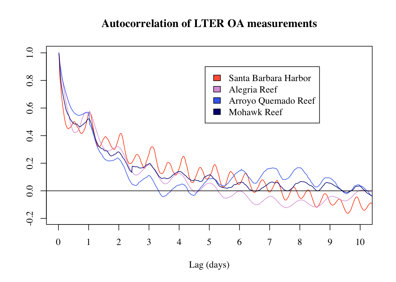
#dev.off()Step 3. Correlation between LTER Sites
Calculate correlation matrix
To determine how much the OA condition co-varies between the four sites, correlation and covariance matrices were constructed on aragonite saturation state measurements. First, seasonal signals were removed in the same method as described above. Then, correlation matrices of aragonite saturation between the four sites were created. Weak relationships were observed, between all sites.
ltercor <- ltermerge

names(ltercor) <- c("Time", "Ale", "Arq", "Mko", "Sbh")

aragcor <- cor(ltercor[,c(2, 3, 4, 5)], use = "pairwise.complete.obs")
View correlation matrix
A main conclusion here is that the SBC LTER sites are not spatially redundant. Another important conclusion from this analysis is that the efficacy of a monitoring network cannot be determined by spatial proximity of monitoring sites alone. Mohawk Reef and Santa Barbara Harbor are geographically very close (less than 3 miles), but this analysis reveals that these two LTER sites have different oceanographic conditions, and that other sites which are much farther away from each other are more similar than Mohawk and Santa Barbara Harbor. Alegria and Arroyo Quemado Reefs are 10 miles apart from each other, and Arroyo Quemado and Mohawk Reefs are 24 miles apart from each other, and each of these pairs share stronger relationships than exists between Santa Barbara Harbor and Mohawk Reef.
| Ale | Arq | Mko | Sbh | |
|---|---|---|---|---|
| Ale | 1.0000000 | 0.3856364 | 0.1137234 | 0.0305191 |
| Arq | 0.3856364 | 1.0000000 | 0.1436457 | 0.3262436 |
| Mko | 0.1137234 | 0.1436457 | 1.0000000 | -0.0688727 |
| Sbh | 0.0305191 | 0.3262436 | -0.0688727 | 1.0000000 |